This page was generated from a Jupyter notebook. You can download the notebook here to run it locally in Jupyter.

Mouse olfactory bulb

Thor reveals cell-resolution mouse olfactory bulb structure.

In this tutorial, we show inference of cell-level spatial gene expression from the Visium spot-level spatial transcriptome and a whole slide image (H&E staining) using Thor.

The spatial transcriptome dataset is the Adult Mouse Olfactory Bulb. The input data can be downloaded from our google drive or 10x Genomics website.

For installation of Thor, please refer to this installation guide.

Import the packages

[1]:

import sys
import os
import logging
import datetime

logger = logging.getLogger()
logger.setLevel(logging.INFO)
logging.basicConfig(format='%(name)s - %(levelname)s - %(message)s')

now = datetime.datetime.now()
logger.info(f"Current Time: {now}")

root - INFO - Current Time: 2023-12-13 12:49:20.893931

[2]:

%config InlineBackend.figure_format = 'retina'

import numpy as np
import pandas as pd
import scanpy as sc
import seaborn as sns
import matplotlib.pyplot as plt
from matplotlib.colors import LinearSegmentedColormap

import warnings

warnings.filterwarnings("ignore")
sc.set_figure_params(scanpy=True, dpi=80, dpi_save=300)
sc.settings.verbosity = 'error'


from thor.pp import WholeSlideImage, Spatial
from thor.finest import fineST
from thor.pl import colors

numexpr.utils - INFO - Note: NumExpr detected 12 cores but "NUMEXPR_MAX_THREADS" not set, so enforcing safe limit of 8.
numexpr.utils - INFO - NumExpr defaulting to 8 threads.

Preprocessing

Preprocessing the whole slide image, including cell segmentation and morphological feature extraction. If not specified, the segmentation data will be saved in a directory (created by Thor) WSI_{sn}.

The WSI can be downloaded directly from google drive.

The outcomes of image preprocessing are two files: - cell mask - cell features

[3]:

sn = 'MOB_10x'
image_path = "Visium_Mouse_Olfactory_Bulb_image.tif"

wsi = WholeSlideImage(image_path, name=sn)

Here we use Cellpose to segment the nuclei. Notice the segmentation can take a long time without GPU. The output file is a n_pixel_row x n_pixel_col matrix.

For the sake of reproducing the results in the paper, we’ll skip this step and load the pre-computed segmentation results from here.

In the downloaded sub-folder (“WSI_MOB_10x”), both the cell segmentation and cell features files are included.

[4]:

%%script echo "Skip cell segmentation"

wsi.process(method='cellpose')

Skip cell segmentation

Preprocessing spatial transcriptome. We used SCANPY to generate an adata for the spots including QC.

We follow the standarized steps used by SCANPY to create the spot adata from the space ranger output directory (st_dir).

The spot adata contains the expression matrix, the location of the spots as pixel positions on the WSI, and the hires, lowres images with scalefactors. - spot.h5ad

You can skip this step and download the files here.The output is in the folder “Spatial_MOB_10x”.

[5]:

st_dir = "10xOlfactory"

trans = Spatial(sn, st_dir)
trans.process_transcriptome(perform_QC=False)

... storing 'feature_types' as categorical
... storing 'genome' as categorical

We can customize the transcriptome preprocessing if needed. Here we do log-normalization.

[6]:

spot_adata_path = trans.spot_adata_path
adata_spot = sc.read_h5ad(spot_adata_path)
sc.pp.normalize_total(adata_spot, target_sum=1e4)
sc.pp.log1p(adata_spot)

adata_spot.write_h5ad(spot_adata_path)

Predicting cell-level gene expression using Markov graph diffusion

After finishing the preprocessing, you should have those files: - The original WSI (image_path) - The cell(nuclei) mask and features (in directory “./WSI_MOB_10x”) - The spot-level gene expression (in directory “./Spatial_MOB_10x”)

[7]:

outdir = os.getcwd()

image_process_dir = os.path.join(outdir, "WSI_MOB_10x")
cell_mask_path = os.path.join(image_process_dir, "cell_mask.npz")
cell_feature_path = os.path.join(image_process_dir, "cell_features.csv")

The first step is to map the spot gene expression to the segmented cells. We use the nearest neighbors approach. This cell-level gene expression is the starting point for the diffusion process.

[8]:

MOB = fineST(
    image_path,
    name=sn,
    spot_adata_path=spot_adata_path,
    cell_features_csv_path=cell_feature_path,
    cell_features_list=['x', 'y', 'mean_gray', 'std_gray', 'entropy_img', 'mean_r', 'mean_g', 'mean_b', 'std_r', 'std_g', 'std_b'],
)

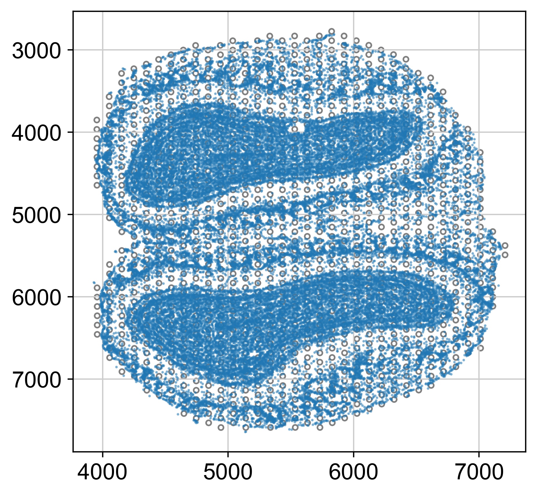
MOB.prepare_input(mapping_margin=2)

[12/13/23 12:49:29] INFO     Thor: Please check alignment of cells and spots
                    INFO     Thor: The first two columns in the node_feat DataFrame need to match the spatial coordinates from obsm['spatial'].
                    INFO     Thor: Mapping cells to the closest spots within 2 x the spot radius

../_images/notebooks_runThor_MOB_18_1.png

[9]:

MOB.adata

[9]:

AnnData object with n_obs × n_vars = 40543 × 32285
    obs: 'in_tissue', 'array_row', 'array_col', 'spot_barcodes', 'x', 'y', 'mean_gray', 'std_gray', 'entropy_img', 'mean_r', 'mean_g', 'mean_b', 'std_r', 'std_g', 'std_b', 'spot_heterogeneity'
    var: 'gene_ids', 'feature_types', 'genome'
    uns: 'log1p', 'spatial', 'cell_image_props'
    obsm: 'spatial'

Second step is set up genes for prediction. For the sake of time, we’ll show prediction of a few genes. The same Markov transition matrix can be applied to all genes. The user-defined genes can be input by either in a 1-column text file or directly as the attribute genes of the MOB object

[10]:

MOB.genes = ['Eomes', 'Uchl1', 'Pcp4l1', 'Col6a1', 'Tbx21', 'Slc17a6', 'Bmp7', 'Camk2a', 'Cystm1', 'Penk', 'Gria1', 'Nap1l5', 'Serpine2', 'Kctd12', 'Pde5a', 'Syt7', 'Vtn']
MOB.set_genes_for_prediction(genes_selection_key=None)
MOB.adata.var[MOB.adata.var['used_for_prediction']]

[10]:

	gene_ids	feature_types	genome	used_for_prediction
Serpine2	ENSMUSG00000026249	Gene Expression	mm10	True
Pcp4l1	ENSMUSG00000038370	Gene Expression	mm10	True
Bmp7	ENSMUSG00000008999	Gene Expression	mm10	True
Pde5a	ENSMUSG00000053965	Gene Expression	mm10	True
Penk	ENSMUSG00000045573	Gene Expression	mm10	True
Uchl1	ENSMUSG00000029223	Gene Expression	mm10	True
Nap1l5	ENSMUSG00000055430	Gene Expression	mm10	True
Slc17a6	ENSMUSG00000030500	Gene Expression	mm10	True
Eomes	ENSMUSG00000032446	Gene Expression	mm10	True
Col6a1	ENSMUSG00000001119	Gene Expression	mm10	True
Gria1	ENSMUSG00000020524	Gene Expression	mm10	True
Vtn	ENSMUSG00000017344	Gene Expression	mm10	True
Tbx21	ENSMUSG00000001444	Gene Expression	mm10	True
Kctd12	ENSMUSG00000098557	Gene Expression	mm10	True
Cystm1	ENSMUSG00000046727	Gene Expression	mm10	True
Camk2a	ENSMUSG00000024617	Gene Expression	mm10	True
Syt7	ENSMUSG00000024743	Gene Expression	mm10	True

In this case study, we include the effect of input spatial transcriptome in constructing the cell-cell network.

Burn in 5 steps using only histology features (vanilla version) for all highly variable genes.
Load the burnin result, perform PCA, and use the transcriptome to adjust the cell-cell network.
The cell-cell network with transcriptome PCA information will be used to perform the production diffusion.

Run time (~ 3 mins on MacbookPro M2)

[11]:

MOB.recipe = 'gene'
MOB.set_params(
    is_rawCount=False,
    out_prefix="fineST",
    write_freq=40,
    n_iter=40,
    conn_csr_matrix="force",
    smoothing_scale=0.8,
    node_features_obs_list=['spot_heterogeneity'],
    n_neighbors=5,
    geom_morph_ratio=0.5,
    geom_constraint=0,
    inflation_percentage=1,
    regulate_expression_mean=False,
    stochastic_expression_neighbors_level='spot',
    smooth_predicted_expression_steps=10,
    reduced_dimension_transcriptome_obsm_key='X_pca',
    adjust_cell_network_by_transcriptome_scale=1,
    n_jobs=4)

MOB.predict_gene_expression()

[12/13/23 12:49:30] INFO     Thor: Using mode gene

Creating piles: 100%|██████████| 4/4 [00:01<00:00,  2.67it/s]

[12/13/23 12:52:17] INFO     Thor: Forcing to recalculate the connectivities.
                    INFO     Thor: Construct SNN with morphological features: ['mean_gray', 'std_gray', 'entropy_img', 'mean_r', 'mean_g', 'mean_b',
                             'std_r', 'std_g', 'std_b'].
                    INFO     Thor: Incorporate the effect of transcriptome.
                    INFO     Thor: Finish constructing SNN
                    INFO     Thor: Add adata.obsp["snn_connectivities"]
                    INFO     Thor: Add adata.obsp["snn_knn_connectivities"]
                    INFO     Thor: Add adata.uns["snn"]
                    INFO     Thor: Weigh cells according to the spot heterogeneity.
                    INFO     Thor: Promote flow of information from more homogeneous cells to less.
                    INFO     Thor: Eliminate low quality edges (<0.1) between cells.
                    INFO     Thor: Compute transition matrix
                    INFO     Thor: self weight scale is set to: 0.200
                    INFO     Thor: Compute transition matrix
                    INFO     Thor: self weight scale is set to: 1.808
[12/13/23 12:52:18] INFO     Thor: Added transition matrix to adata.obsp["snn_transition_matrix"]

... storing 'spot_barcodes' as categorical

                    INFO     Thor: fineST estimation starts.
[12/13/23 12:52:34] INFO     Thor: fineST estimation finished.

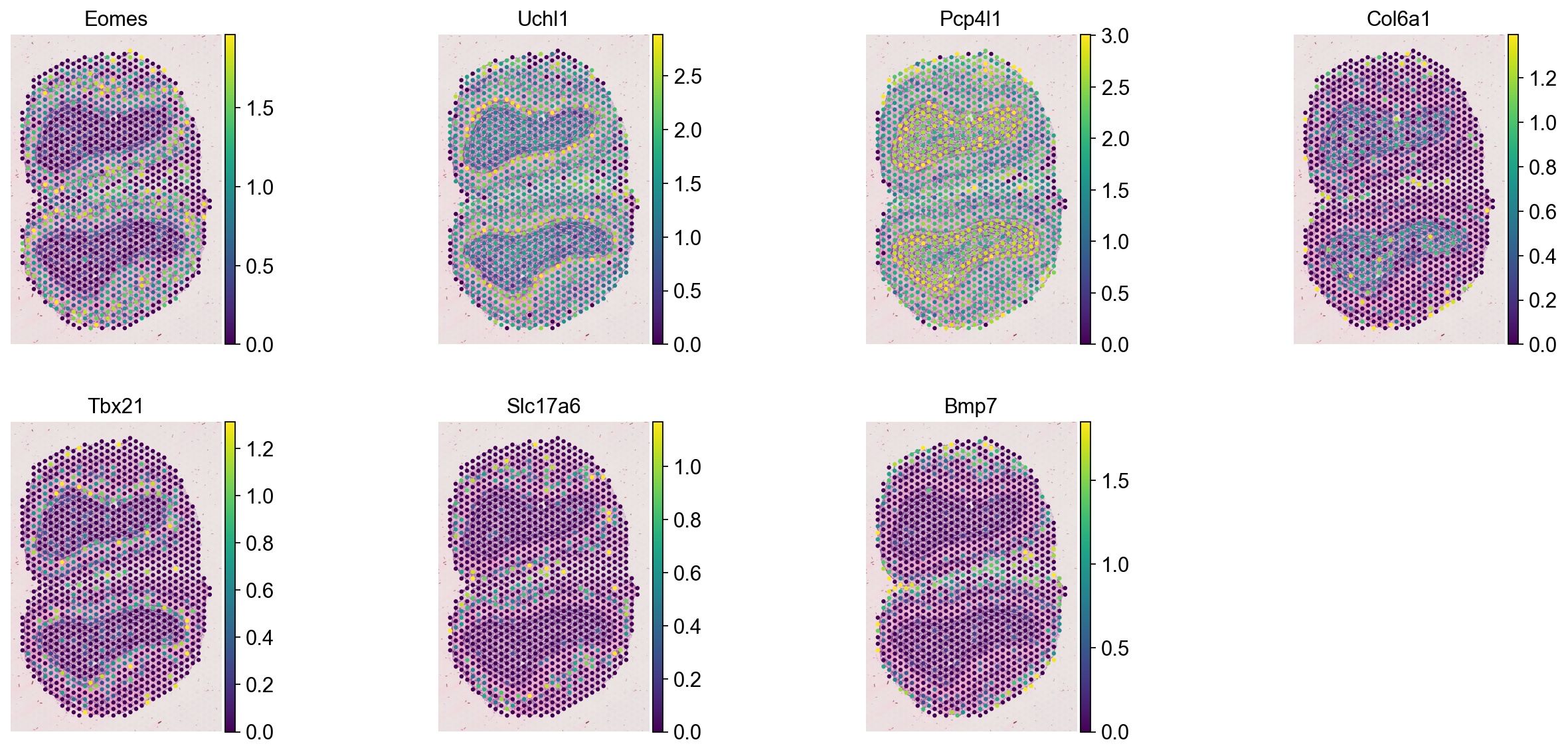
Check the expression of a few genes.

[12]:

ad_thor = MOB.load_result('fineST_40_samp10.npz')
ad_thor

[12]:

AnnData object with n_obs × n_vars = 40543 × 17
    obs: 'in_tissue', 'array_row', 'array_col', 'spot_barcodes', 'x', 'y', 'mean_gray', 'std_gray', 'entropy_img', 'mean_r', 'mean_g', 'mean_b', 'std_r', 'std_g', 'std_b', 'spot_heterogeneity', 'node_weights'
    var: 'gene_ids', 'feature_types', 'genome', 'used_for_prediction', 'used_for_reduced', 'used_for_vae', 'highly_variable', 'means', 'dispersions', 'dispersions_norm'
    uns: 'log1p', 'spatial', 'cell_image_props', 'hvg', 'snn'
    obsm: 'spatial', 'X_pca'
    obsp: 'snn_connectivities', 'snn_knn_connectivities', 'snn_transition_matrix'

[13]:

genes = ['Eomes', 'Uchl1', 'Pcp4l1', 'Col6a1', 'Tbx21', 'Slc17a6', 'Bmp7']

ad_spot = sc.read_h5ad(spot_adata_path)
sc.pl.spatial(ad_spot, color=genes, vmax='p99', frameon=False, ncols=4)

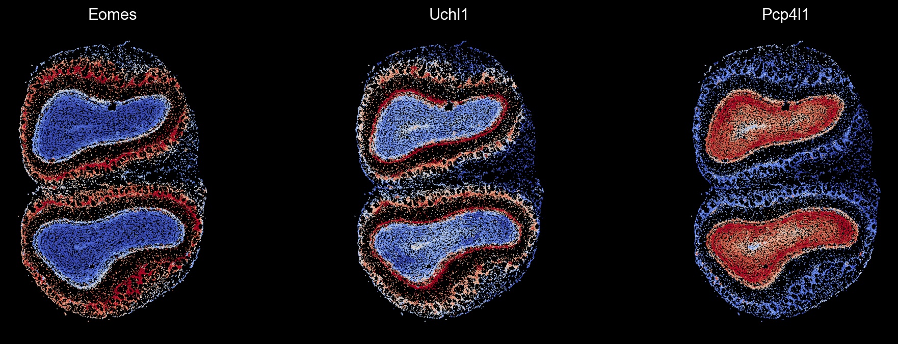
../_images/notebooks_runThor_MOB_26_0.png

[14]:

genes = ['Eomes', 'Uchl1', 'Pcp4l1']

sc.set_figure_params(scanpy=True, dpi=80, dpi_save=100, facecolor='k', frameon=False)
fw2 = LinearSegmentedColormap.from_list('fw2', colors.continuous_palettes['fireworks2'])

fig, axes = plt.subplots(1, 3, figsize=(15, 5))
i = 0

for gene in genes:
    sc.pl.spatial(ad_thor, color=gene, spot_size=15, vmin='p5', vmax='p95', colorbar_loc=None, cmap='coolwarm', img_key=None, show=False, ax=axes[i])
    axes[i].set_title(gene, color='w')
    i += 1
plt.show()

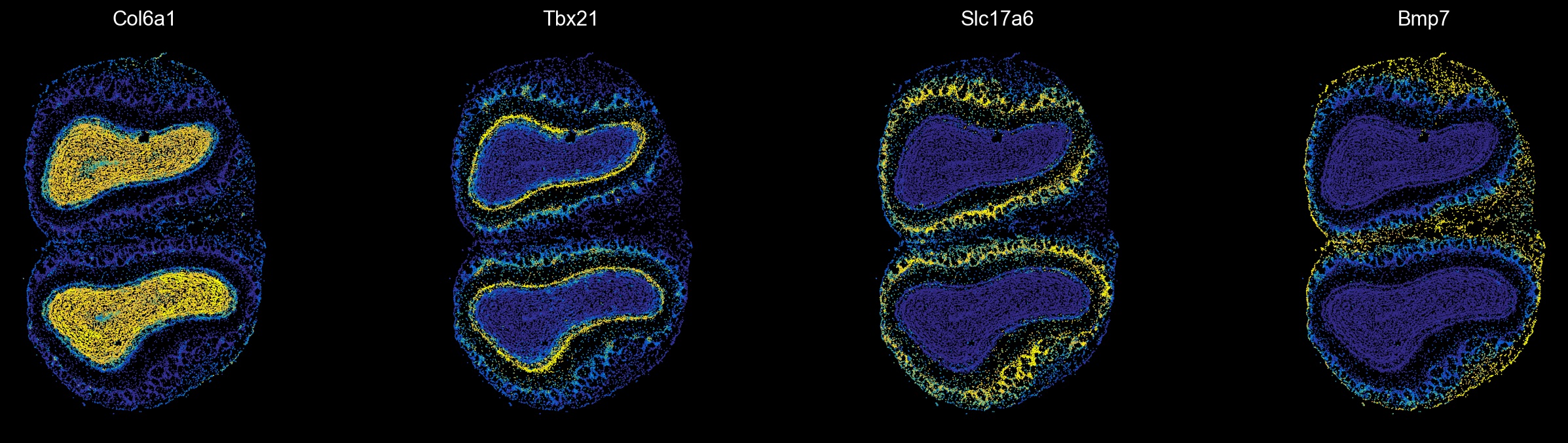
../_images/notebooks_runThor_MOB_27_0.png

Visualize module-specific genes

[15]:

from matplotlib.colors import LinearSegmentedColormap
from thor.pl import colors

mod_genes = ['Col6a1', 'Tbx21', 'Slc17a6', 'Bmp7']


sc.set_figure_params(scanpy=True, dpi=80, dpi_save=100, facecolor='k', frameon=False)
yb = LinearSegmentedColormap.from_list('yb', colors.continuous_palettes['blueYellow'])

fig, axes = plt.subplots(1, 4, figsize=(20, 5))
i = 0

for gene in mod_genes:
    sc.pl.spatial(ad_thor, color=gene, spot_size=15, vmin='p2', vmax='p98', colorbar_loc=None, cmap=yb, img_key=None, show=False, ax=axes[i])
    axes[i].set_title(gene, color='w')
    i += 1
plt.show()

../_images/notebooks_runThor_MOB_29_0.png

[ ]: