Ductal carcinoma in situ
Thor performs unbiased screening of breast cancer hallmarks in Ductal Carcinoma in situ sample and reveals heterogeneity of immune response.
Run Thor
In this tutorial, we show inference of cell-level spatial gene expression from the Visium spot-level spatial transcriptome and a whole slide image (H&E staining) using Thor.
The spatial dataset is Human Breast Cancer: Ductal Carcinoma In Situ, Invasive Carcinoma (FFPE). The input data are downloaded from 10x Genomics website.
Thor processed data can be downloaded directly from google drive.
For installation of Thor, please refer to this installation guide.
Import the packages
[1]:
import sys
import os
import logging
import datetime

logger = logging.getLogger()
logger.setLevel(logging.INFO)
logging.basicConfig(format='%(name)s - %(levelname)s - %(message)s')

now = datetime.datetime.now()
logger.info(f"Current Time: {now}")
root - INFO - Current Time: 2023-12-13 16:53:16.118962
[2]:
%config InlineBackend.figure_format = 'retina'


import numpy as np
import pandas as pd
import scanpy as sc
import seaborn as sns
import matplotlib.pyplot as plt
sc.set_figure_params(scanpy=True, dpi=80, dpi_save=300)
sc.settings.verbosity = 'error'


from thor.pp import WholeSlideImage, Spatial
from thor.finest import fineST
numexpr.utils - INFO - Note: NumExpr detected 12 cores but "NUMEXPR_MAX_THREADS" not set, so enforcing safe limit of 8.
numexpr.utils - INFO - NumExpr defaulting to 8 threads.
Preprocessing
Preprocessing the whole slide image, including cell segmentation and morphological feature extraction. If not specified, the segmentation data will be saved in a directory (created by Thor) WSI_{sn}.
The WSI can be downloaded directly from google drive.
The outcomes are: cell mask and the cell feature.csv
[3]:
sn = 'DCIS_10x'
image_path = "Visium_FFPE_Human_Breast_Cancer_image.tif"

wsi = WholeSlideImage(image_path, name=sn)
Here we use Cellpose to segment the nuclei. Notice the segmentation can take a long time without GPU. The output file is a n_pixel_row x n_pixel_col matrix. We’ll skip this step and load the pre-computed segmentation results from here.
[4]:
%%script echo "Skip cell segmentation"

wsi.process(method='cellpose')
Skip cell segmentation
Extract handcrafted image features based on the image and nuclei segmentation result.
[5]:
cell_mask_path = os.path.join('WSI_DCIS_10x', 'cell_mask.npz')
wsi = WholeSlideImage(image_path, name=sn, nuclei_seg_path=cell_mask_path, nuclei_seg_format='mask_array_npz')
wsi.process()
[12/13/23 16:53:37] INFO     Thor: 76396 cells detected.
                    INFO     Thor: 76396 cells mapped to spots.
[12/13/23 16:53:38] INFO     Thor: 76359 cells kept.
<function mean at 0x107c40900>
                    INFO     Thor: Extracting image features from a square image patch of size 112 pixels centered at the cell.
Extracting gray image features: 100%|██████████| 76359/76359 [00:04<00:00, 16574.04it/s]
Extracting RGB features: 100%|██████████| 76359/76359 [00:33<00:00, 2297.83it/s]
Preprocessing spatial transcriptome. We used SCANPY to generate an adata for the spots including QC.
We follow the standarized steps used by SCANPY to create the spot adata from the space ranger output directory (visium_dir). The spot adata contains the expression matrix, the location of the spots as pixel positions on the WSI, and the hires, lowres images with scalefactors. - spot.h5ad
We skip this step here and the files can be downloaded from here
Predicting cell-level gene expression using Thor diffusion
After finishing the preprocessing, you should have those files: - The original WSI (image_path) - The cell(nuclei) mask and features (in directory “./WSI_DCIS_10x”) - The spot-level gene expression (in directory “./Spatial_DCIS_10x”)
[6]:
outdir = os.getcwd()

image_process_dir = os.path.join(outdir, "WSI_DCIS_10x")
cell_mask_path = os.path.join(image_process_dir, "cell_mask.npz")
cell_feature_path = os.path.join(image_process_dir, "cell_features.csv")

spatial_dir = os.path.join(outdir, "Spatial_DCIS_10x")
spot_adata_path = os.path.join(spatial_dir, "spot.h5ad")
The first step is to map the spot gene expression to the segmented cells. We use the nearest neighbors approach. This cell-level gene expression is the starting point for the diffusion process.
[7]:
DCIS = fineST(
    image_path,
    name="DCIS_10x",
    spot_adata_path=spot_adata_path,
    cell_features_csv_path=cell_feature_path
)

DCIS.prepare_input(mapping_margin=10)
[12/13/23 16:54:25] INFO     Thor: Please check alignment of cells and spots
                    INFO     Thor: The first two columns in the node_feat DataFrame need to match the spatial coordinates from obsm['spatial'].
                    INFO     Thor: Mapping cells to the closest spots within 10 x the spot radius
[8]:
DCIS.adata
[8]:
AnnData object with n_obs × n_vars = 76344 × 16784
    obs: 'in_tissue', 'array_row', 'array_col', 'n_genes', 'n_genes_by_counts', 'total_counts', 'total_counts_mt', 'pct_counts_mt', 'spot_barcodes', 'x', 'y', 'mean_gray', 'std_gray', 'entropy_img', 'mean_r', 'mean_g', 'mean_b', 'std_r', 'std_g', 'std_b', 'spot_heterogeneity'
    var: 'gene_ids', 'feature_types', 'genome', 'n_cells', 'mt', 'n_cells_by_counts', 'mean_counts', 'pct_dropout_by_counts', 'total_counts'
    uns: 'spatial', 'cell_image_props'
    obsm: 'spatial'
There are 75117 cells and for the sake of time, we’ll show prediction of a few genes. The same Markov transition matrix can be applied to all genes. The user-defined genes can be input by either in a 1-column text file or directly as an attribute of the DCIS object
[9]:
DCIS.genes = ['VEGFA', 'FGFR4', 'TPD52', 'GRB7', 'JUP', 'SCGB2A2', 'KANK1', 'ESR1', 'TFRC', 'ERBB2']

DCIS.set_genes_for_prediction(genes_selection_key=None)
[10]:
DCIS.adata.var[DCIS.adata.var['used_for_prediction']]
[10]:
| gene_ids | feature_types | genome | n_cells | mt | n_cells_by_counts | mean_counts | pct_dropout_by_counts | total_counts | used_for_prediction | |
|---|---|---|---|---|---|---|---|---|---|---|
| TFRC | ENSG00000072274 | Gene Expression | GRCh38 | 1847 | False | 1847 | 2.779190 | 26.648133 | 6998.0 | True |
| FGFR4 | ENSG00000160867 | Gene Expression | GRCh38 | 165 | False | 165 | 0.094122 | 93.447180 | 237.0 | True |
| VEGFA | ENSG00000112715 | Gene Expression | GRCh38 | 1900 | False | 1900 | 3.851866 | 24.543288 | 9699.0 | True |
| ESR1 | ENSG00000091831 | Gene Expression | GRCh38 | 166 | False | 166 | 0.069102 | 93.407466 | 174.0 | True |
| TPD52 | ENSG00000076554 | Gene Expression | GRCh38 | 2016 | False | 2016 | 5.621922 | 19.936458 | 14156.0 | True |
| KANK1 | ENSG00000107104 | Gene Expression | GRCh38 | 818 | False | 818 | 0.499603 | 67.513900 | 1258.0 | True |
| SCGB2A2 | ENSG00000110484 | Gene Expression | GRCh38 | 2213 | False | 2213 | 17.403097 | 12.112788 | 43821.0 | True |
| ERBB2 | ENSG00000141736 | Gene Expression | GRCh38 | 2417 | False | 2417 | 22.986498 | 4.011120 | 57880.0 | True |
| GRB7 | ENSG00000141738 | Gene Expression | GRCh38 | 1411 | False | 1411 | 2.008737 | 43.963463 | 5058.0 | True |
| JUP | ENSG00000173801 | Gene Expression | GRCh38 | 1758 | False | 1758 | 2.829230 | 30.182685 | 7124.0 | True |
[11]:
DCIS.recipe = 'gene'
DCIS.set_params(
    is_rawCount=False,
    out_prefix="fineST",
    write_freq=10,
    n_iter=20,
    conn_csr_matrix="force",
    smoothing_scale=0.8,
    node_features_obs_list=['spot_heterogeneity'],
    n_neighbors=5,
    geom_morph_ratio=1,
    geom_constraint=0,
    inflation_percentage=None,
    regulate_expression_mean=False,
    stochastic_expression_neighbors_level='spot',
    smooth_predicted_expression_steps=1,
    reduced_dimension_transcriptome_obsm_key=None,
    adjust_cell_network_by_transcriptome_scale=0,
    n_jobs=4)
[12]:
DCIS.predict_gene_expression()
[12/13/23 16:54:27] INFO     Thor: Using mode gene
                    INFO     Thor: Forcing to recalculate the connectivities.
                    INFO     Thor: Construct SNN with morphological features: ['mean_gray', 'std_gray', 'entropy_img', 'mean_r', 'mean_g', 'mean_b',
                             'std_r', 'std_g', 'std_b'].
[12/13/23 16:54:28] INFO     Thor: Finish constructing SNN
                    INFO     Thor: Add adata.obsp["snn_connectivities"]
                    INFO     Thor: Add adata.obsp["snn_knn_connectivities"]
                    INFO     Thor: Add adata.uns["snn"]
                    INFO     Thor: Weigh cells according to the spot heterogeneity.
[12/13/23 16:54:29] INFO     Thor: Promote flow of information from more homogeneous cells to less.
                    INFO     Thor: Eliminate low quality edges (<0.1) between cells.
                    INFO     Thor: Compute transition matrix
                    INFO     Thor: self weight scale is set to: 0.200
                    INFO     Thor: Added transition matrix to adata.obsp["snn_transition_matrix"]
... storing 'spot_barcodes' as categorical
[12/13/23 16:54:30] INFO     Thor: fineST estimation starts.
[12/13/23 16:54:48] INFO     Thor: fineST estimation finished.
Check the expression of a few genes.
[13]:
ad_thor = DCIS.load_result('fineST_20_samp1.npz')
ad_thor
[13]:
AnnData object with n_obs × n_vars = 76344 × 10
    obs: 'in_tissue', 'array_row', 'array_col', 'n_genes', 'n_genes_by_counts', 'total_counts', 'total_counts_mt', 'pct_counts_mt', 'spot_barcodes', 'x', 'y', 'mean_gray', 'std_gray', 'entropy_img', 'mean_r', 'mean_g', 'mean_b', 'std_r', 'std_g', 'std_b', 'spot_heterogeneity', 'node_weights'
    var: 'gene_ids', 'feature_types', 'genome', 'n_cells', 'mt', 'n_cells_by_counts', 'mean_counts', 'pct_dropout_by_counts', 'total_counts', 'used_for_prediction', 'used_for_reduced', 'used_for_vae'
    uns: 'spatial', 'cell_image_props', 'snn'
    obsm: 'spatial'
    obsp: 'snn_connectivities', 'snn_knn_connectivities', 'snn_transition_matrix'
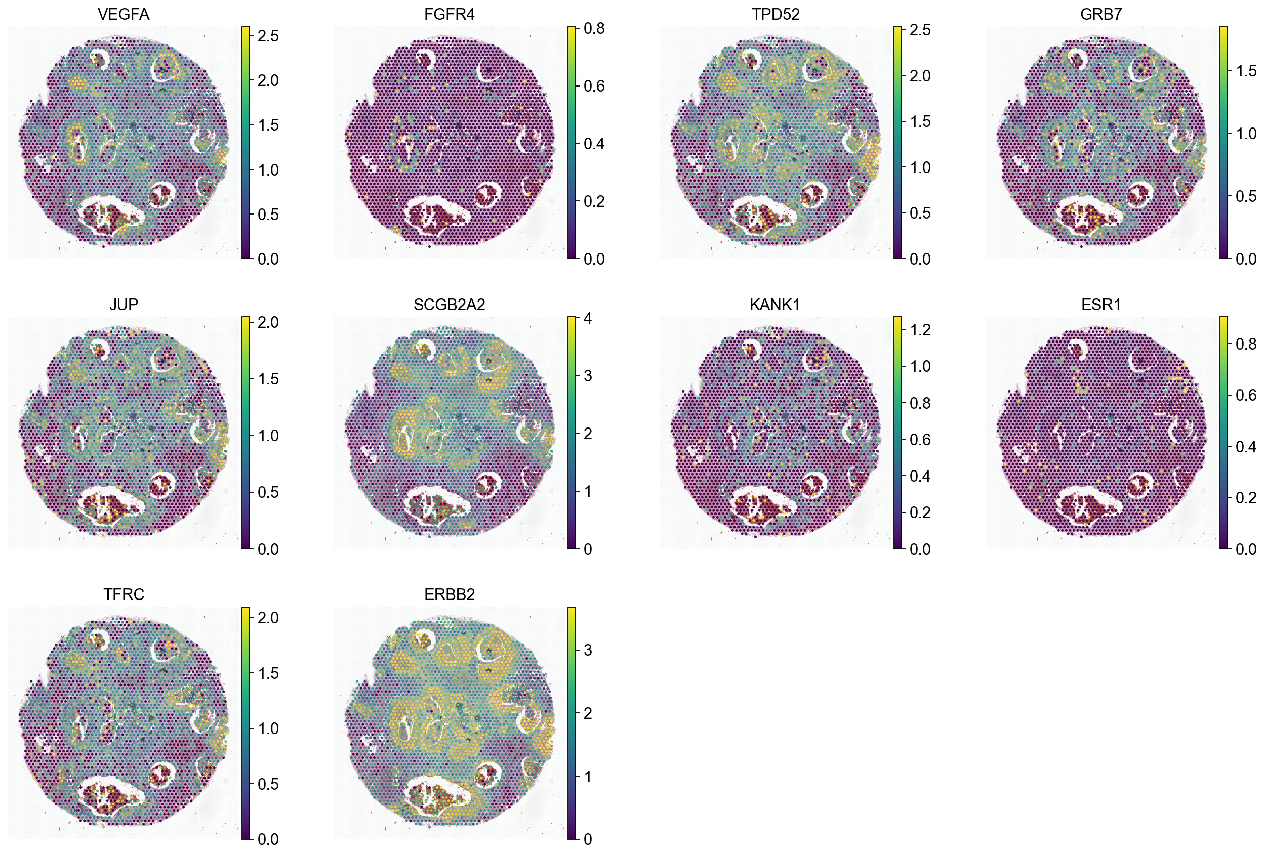
[14]:
genes = DCIS.genes

ad_spot = sc.read_h5ad(spot_adata_path)
sc.pl.spatial(ad_spot, color=genes, vmax='p99', frameon=False)
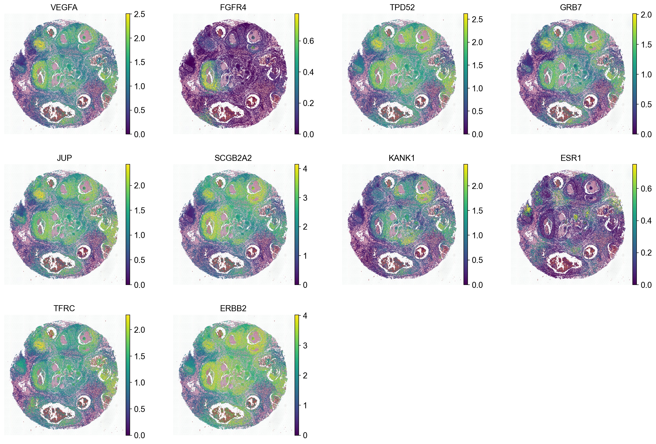
[15]:
genes = DCIS.genes
sc.pl.spatial(ad_thor, color=genes, spot_size=50, vmax='p99', frameon=False)
Advance analysis
In this notebook, we’ll perform analyses on the Ductal Carcinoma In Situ (DCIS) spatial data at cell-level inferred by Thor, as follows,
Visualization of genes in the physical context at cell level
Tumor activity using oncogenes and tumor suppressor genes
Hallmark pathway enrichment
Copy number variation calculation
Tertiary Lymphoid Structures quantification
For installation of Thor, please refer to Thor website.
The cell-level expression of the highly variable genes (2747 genes) inferred by Thor can be downloaded from the link. You can also download the nuclei segmentation masks and full resolution image in the same link if you skip first part of the notebooks in this case study.
Import packages
[16]:
import os
import scanpy as sc
import numpy as np
from scipy import stats
import seaborn as sns
import matplotlib as mpl
from matplotlib import pyplot as plt
from PIL import Image
from shapely.geometry import Polygon


import thor
from thor.utils import convert_pixel_to_micron_visium, get_ROI_tuple_from_polygon, get_adata_layer_array
from thor.pl import annotate_ROI, get_nuclei_pixels, single_molecule
from thor.analy import get_pathway_score
[17]:
%config InlineBackend.figure_format = 'retina'
sc.set_figure_params(scanpy=True, dpi=80, dpi_save=300)
sc.settings.verbosity = "error"
Load the image (for visualization) and Thor-predicted cell-level transcriptome result
[18]:
image_path = "Visium_FFPE_Human_Breast_Cancer_image.tif"
fullres_im = np.array(Image.open(image_path))

adata_path = os.path.join("Thor_DCIS_10x", "cell_data_thor.h5ad")
ad = sc.read_h5ad(adata_path)
ad
[18]:
AnnData object with n_obs × n_vars = 76320 × 2748
    obs: 'in_tissue', 'array_row', 'array_col', 'n_genes', 'n_genes_by_counts', 'total_counts', 'total_counts_mt', 'pct_counts_mt', 'spot_barcodes', 'x', 'y', 'mean_gray', 'std_gray', 'entropy_img', 'mean_r', 'mean_g', 'mean_b', 'std_r', 'std_g', 'std_b', 'spot_heterogeneity', 'node_weights', 'tumor_region', 'tumor_region_ext', 'copy_variation'
    var: 'gene_ids', 'feature_types', 'genome', 'n_cells', 'mt', 'n_cells_by_counts', 'mean_counts', 'pct_dropout_by_counts', 'total_counts', 'used_for_prediction', 'used_for_reduced', 'used_for_vae'
    uns: 'cell_image_props', 'copy_variation_colors', 'hvg', 'leiden', 'leiden_colors', 'neighbors', 'pca', 'recluster_normal_colors', 'snn', 'spatial', 'tumor_cluster_CNV_colors', 'tumor_normal_subtumor_colors', 'tumor_region_boundaries', 'umap'
    obsm: 'spatial'
    obsp: 'snn_connectivities', 'snn_knn_connectivities', 'snn_transition_matrix'
Visualize genes at tissue and cell level
[19]:
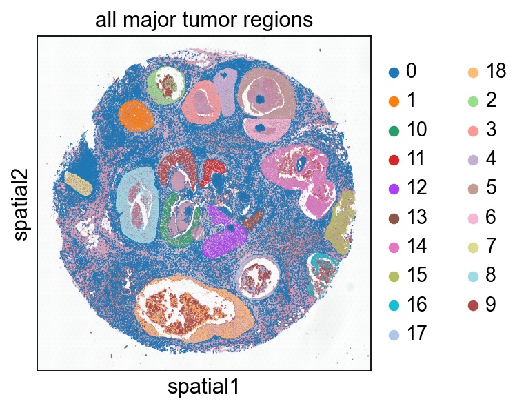
# Show all the tumor regions
# '0' means non-tumor
sc.pl.spatial(ad, color='tumor_region', spot_size=50, cmap='tab20b', title='all major tumor regions')
[20]:
palette = thor.pl.colors.continuous_palettes['blueYellow']
cmap = mpl.colors.LinearSegmentedColormap.from_list('my_cmap', palette, N=256)
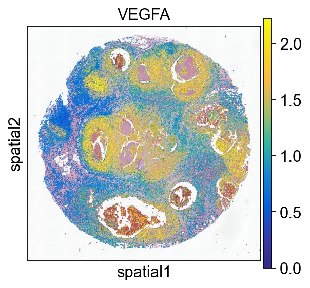
[21]:
gene = 'VEGFA'
sc.pl.spatial(ad, color='VEGFA', spot_size=50, vmax='p99', cmap=cmap)
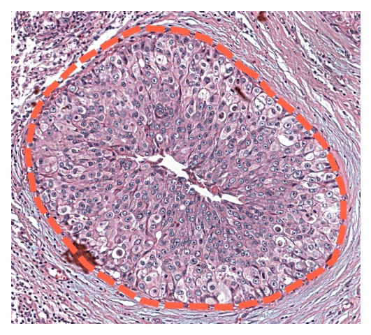
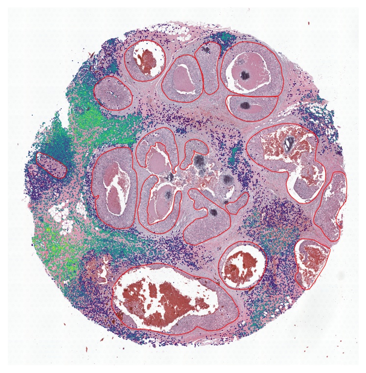
Close-up gene expression in cells can be seamlessly explored using our dedicated webapp Mjolnir or as static figures plotted using Thor’s plotting functions. Here we annotate tumor regions on the H & E image according to Agoko NV, Belgium on 10x Genomics website.
We then use Mjolnir to extract the tumor regions and gene expression matrices of the cells in those regions.
[22]:
tumor1 = ad.uns['tumor_region_boundaries']['1']
tumor1_polygon = Polygon(tumor1)
ROI_tuple = get_ROI_tuple_from_polygon(tumor1, extend_pixels=100)
annotate_ROI(fullres_im, ROI_polygon=tumor1_polygon, lw=4)
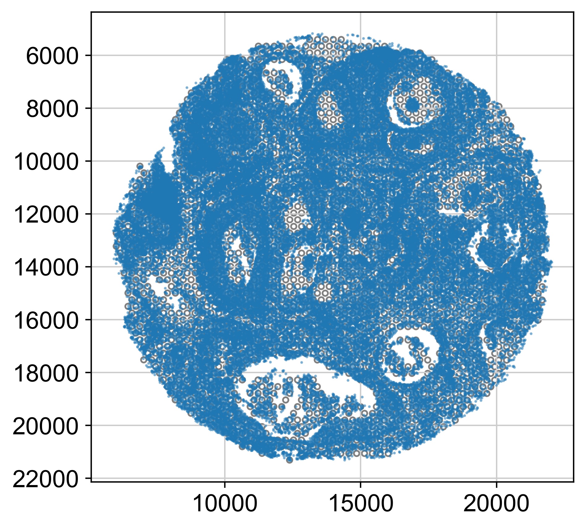
load the cellmasks
[23]:
cells_pixels = get_nuclei_pixels(ad, "WSI_DCIS_10x/cell_mask.npz")
microPerPixel = convert_pixel_to_micron_visium(ad)
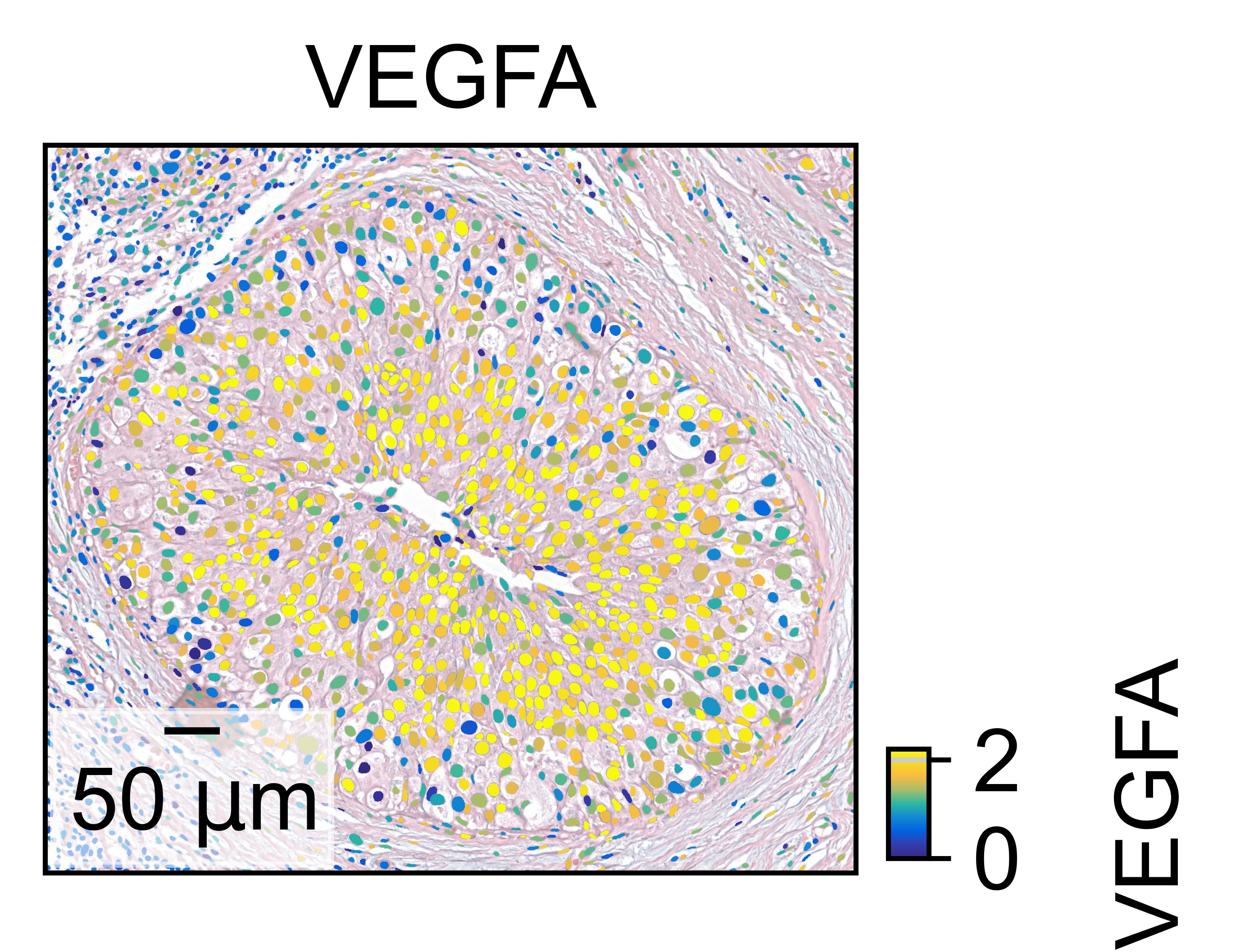
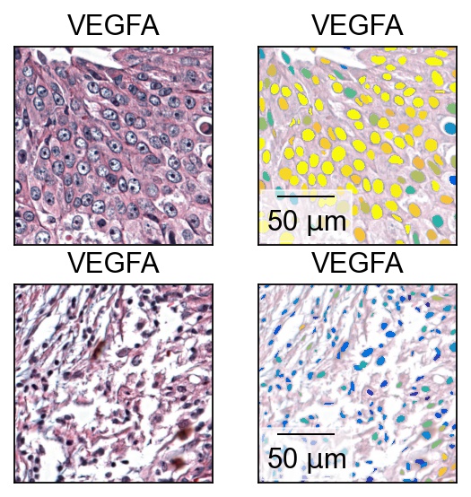
[24]:
gene = 'VEGFA'
expression_vector = get_adata_layer_array(ad[:, gene])

ax = single_molecule(gene, expression_vector, cells_pixels, full_res_im=fullres_im, ROI_tuple=ROI_tuple, cmap=cmap, img_alpha=0.5, vmax='p99', dpi=500, figsize=(2,2))
thor.plotting.fill.add_scalebar(ax, microPerPixel, 'um', 'lower left')
[25]:
ROI_squares = [[9000, 7900, 500, 500], [10400, 8900, 500, 500]]

fig, axes = plt.subplots(2, 2)

i = 1
for r in ROI_squares:
    single_molecule(gene, expression_vector, cells_pixels, full_res_im=fullres_im, ROI_tuple=r, img_alpha=1, figsize=(3, 3), dpi=200, alpha=0, show_cbar=False, return_fig=False, show=False, cmap=cmap, ax=axes[i, 0])
    ax=single_molecule(gene, expression_vector, cells_pixels, full_res_im=fullres_im, ROI_tuple=r, img_alpha=0.5, figsize=(3, 3), dpi=200, alpha=1, show_cbar=False, return_fig=False, show=False, cmap=cmap, vmax='p99', ax=axes[i, 1])
    thor.plotting.fill.add_scalebar(ax, microPerPixel, 'um', 'lower left')
    i = i - 1
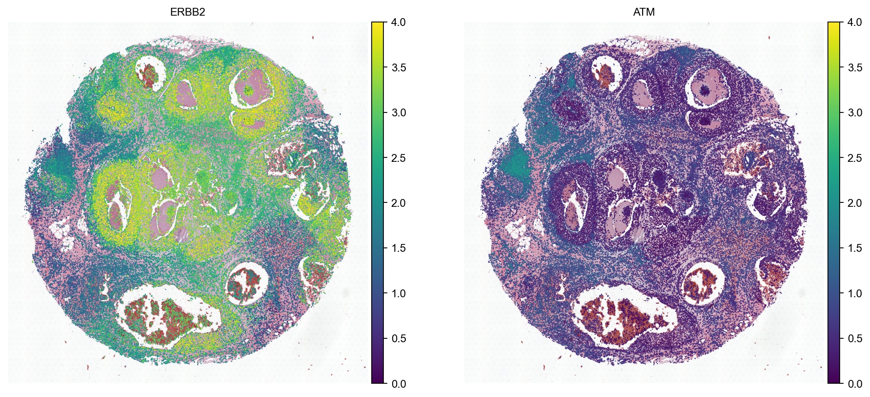
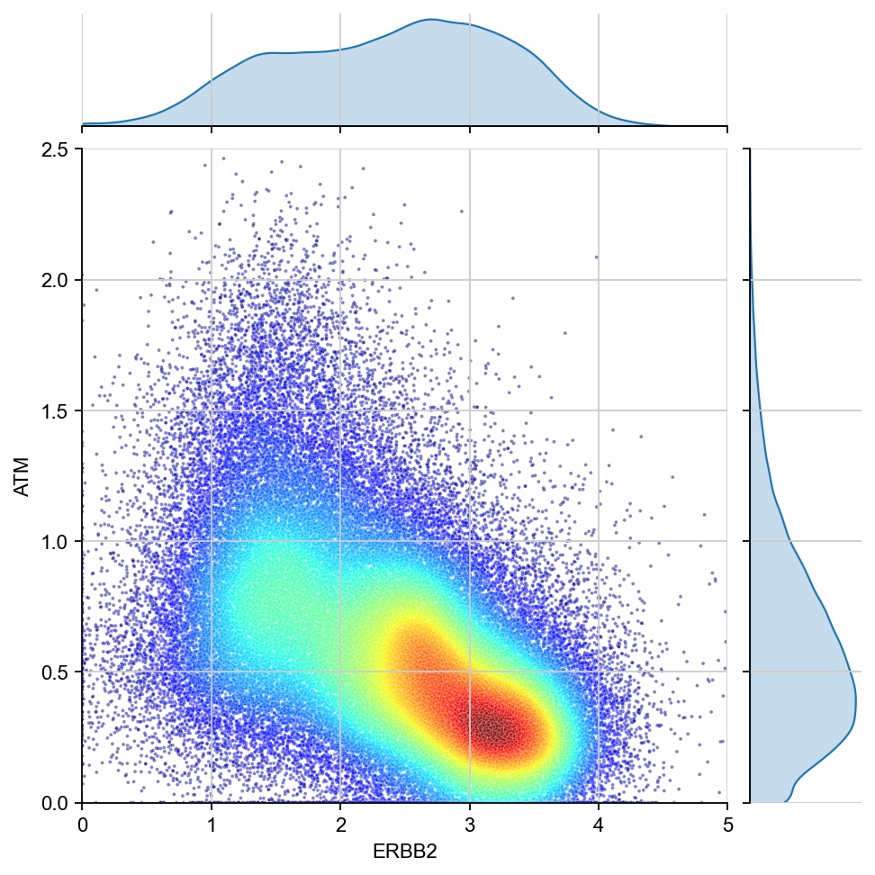
Expression profile of oncogene and tumor suppressor gene
[26]:
sc.set_figure_params(dpi=80, vector_friendly=True, fontsize=10, frameon=False, figsize=(6,6))
sc.pl.spatial(ad, color=["ERBB2", "ATM"], spot_size=50, vmax=4, cmap='viridis', img_key="hires", show=False)
[26]:
[<Axes: title={'center': 'ERBB2'}, xlabel='spatial1', ylabel='spatial2'>,
 <Axes: title={'center': 'ATM'}, xlabel='spatial1', ylabel='spatial2'>]
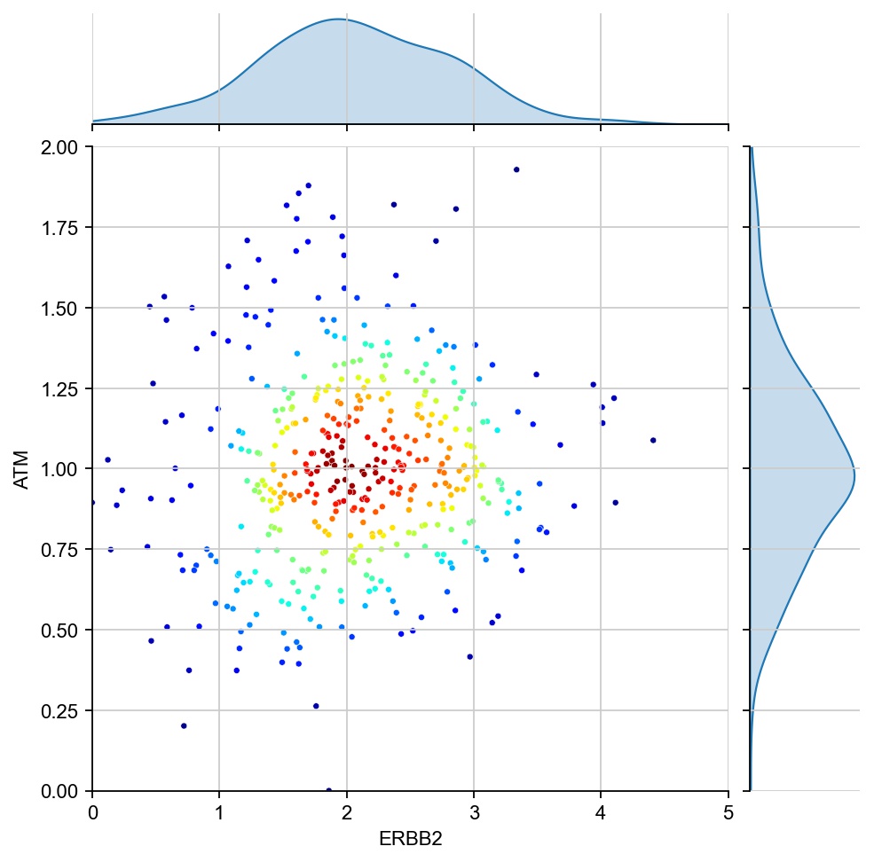
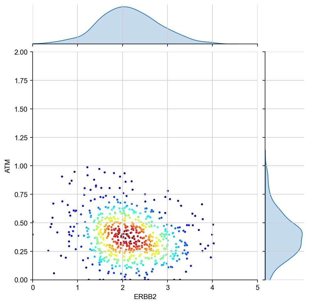
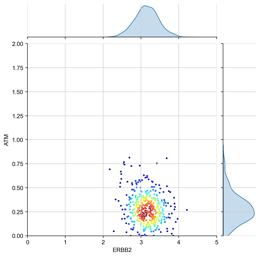
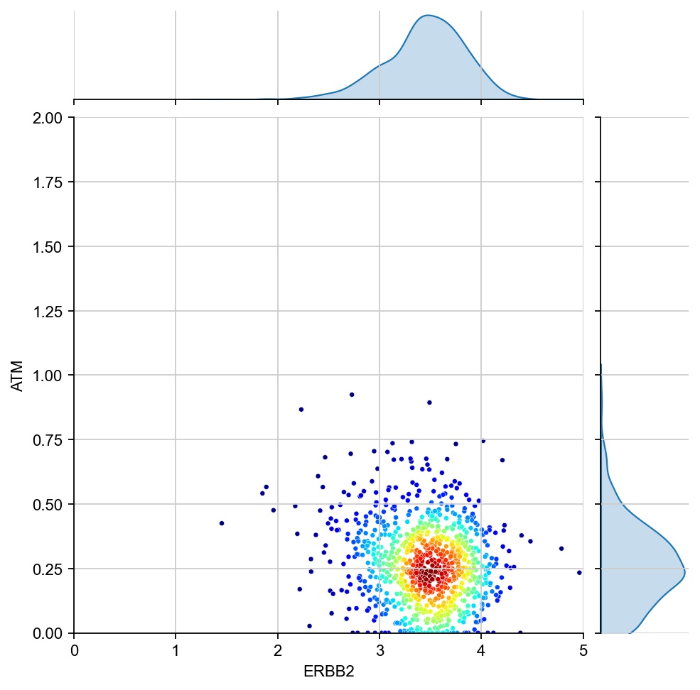
[27]:
g1 ="ERBB2"
g2 = "ATM"
region_col = "tumor_region"
for region in ["7", "1", "17", "11", "6", "15"]:

    x = ad[ad.obs[region_col]==region, g1].X[:, 0]
    y = ad[ad.obs[region_col]==region, g2].X[:, 0]

    values = np.vstack([x, y])
    kernel = stats.gaussian_kde(values)(values)
    ax1 = sns.jointplot(x=x, y=y, kind="kde", fill=True, levels=100)

    ax1.ax_joint.cla()
    plt.sca(ax1.ax_joint)
    ax = sns.scatterplot(x=x, y=y, s=10, alpha=1, c=kernel, cmap="jet", ax=ax1.ax_joint)
    ax.set_xlabel(g1)
    ax.set_ylabel(g2)
    ax.set_xlim(0, 5)
    ax.set_ylim(0, 2)
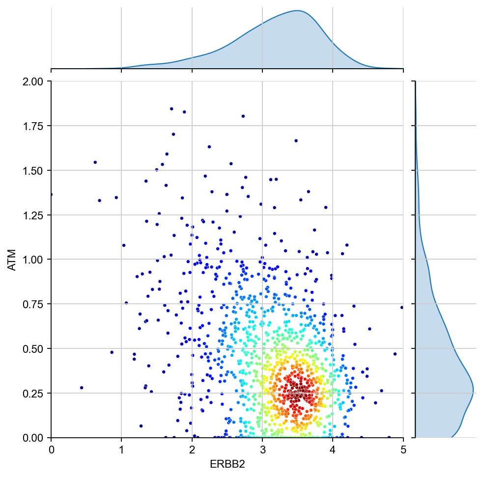
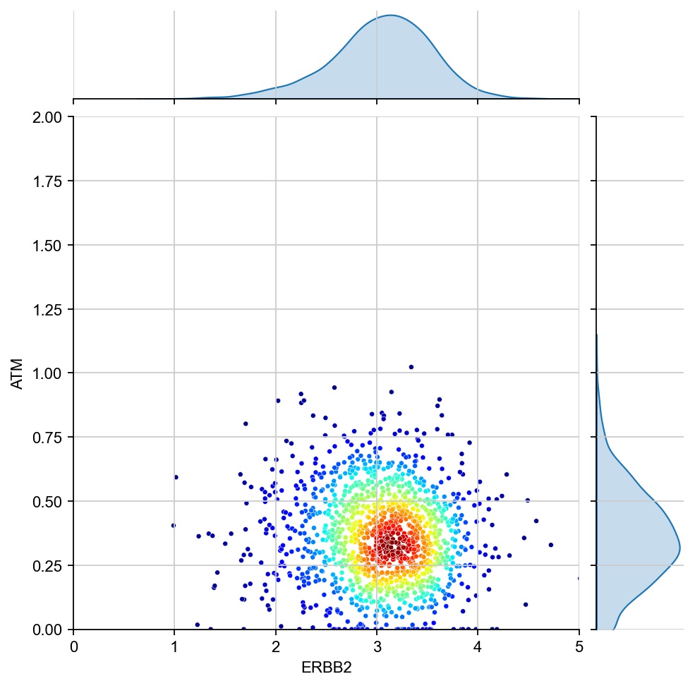
[28]:
g1 ="ERBB2"
g2 = "ATM"

x = ad[:, g1].X[:, 0]
y = ad[:, g2].X[:, 0]

values = np.vstack([x, y])
kernel = stats.gaussian_kde(values)(values)
ax1 = sns.jointplot(x=x, y=y, kind="kde", fill=True, levels=100)

ax1.ax_joint.cla()
plt.sca(ax1.ax_joint)
ax = sns.scatterplot(x=x, y=y, s=3, alpha=0.5, c=kernel, cmap="jet", ax=ax1.ax_joint)
ax.set_xlabel(g1)
ax.set_ylabel(g2)
ax.set_xlim(0, 5)
ax.set_ylim(0, 2.5)

plt.show()
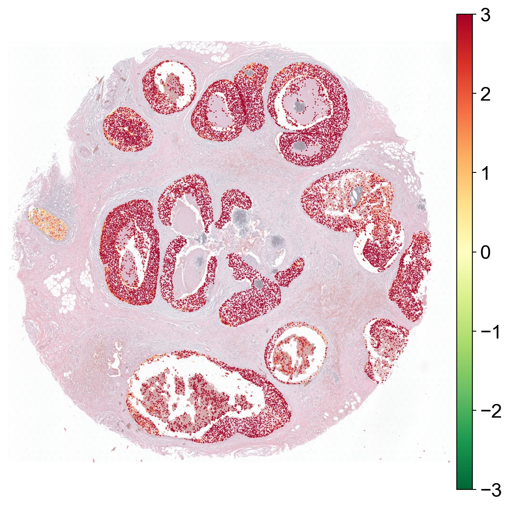
[29]:
g1 ="ERBB2"
g2 = "ATM"
region_col = "tumor_region"

x = ad[:, g1].X[:, 0]
y = ad[:, g2].X[:, 0]

ad.obs['severe'] = np.log2(x/(y+0.01))

# tumor_region '0' is the background (non-tumor) region
ad1 = ad[ad.obs[region_col] != '0']

sc.set_figure_params(dpi=80, color_map="RdYlGn_r", vector_friendly=True, fontsize=18, frameon=False, figsize=(8,8))
sc.pl.spatial(ad1, color=["severe"], spot_size=40, vmin=-3, vmax=3, alpha_img=0.5, title="")
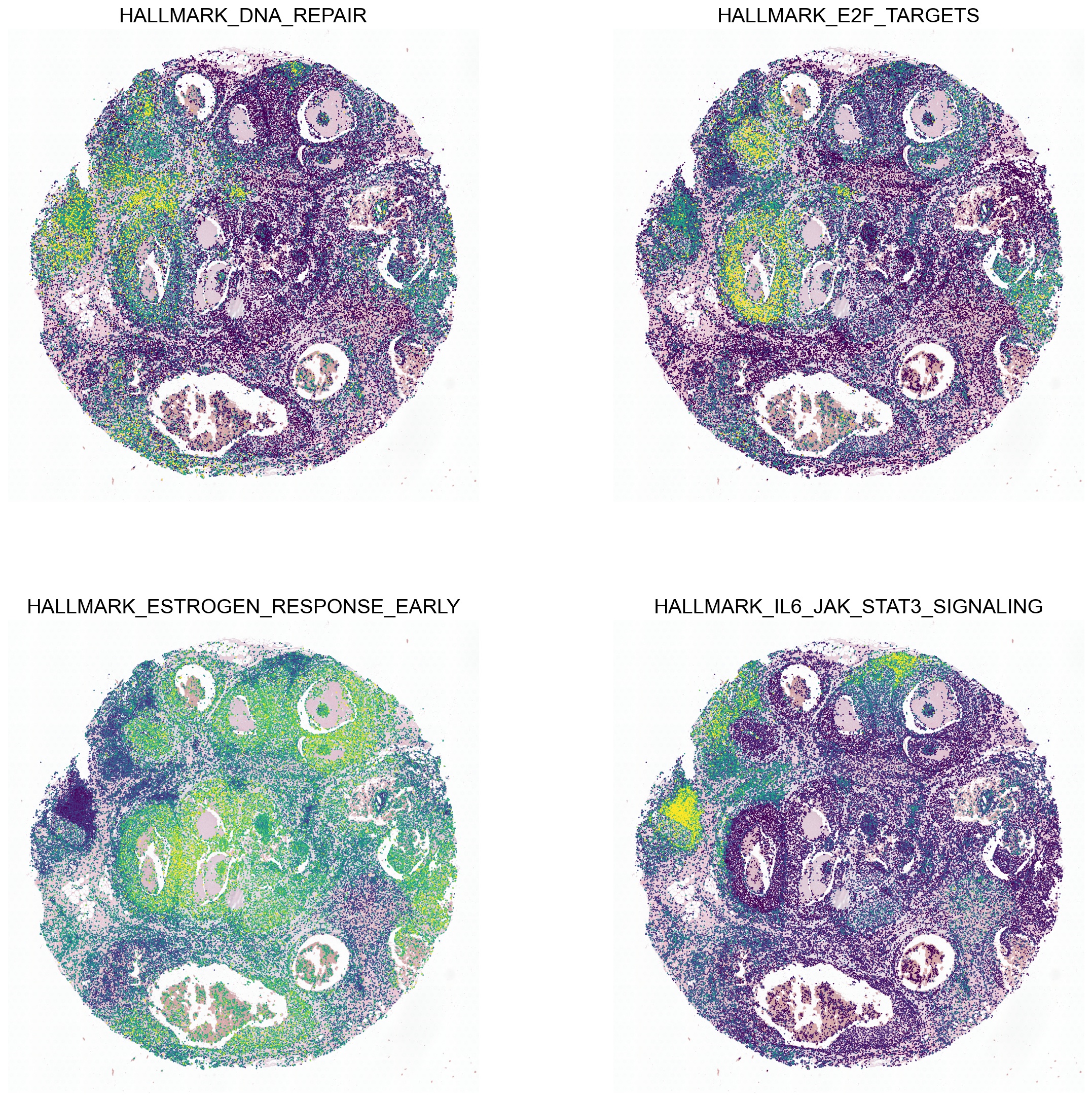
Hallmark pathway enrichment
Pathway enrichment analyses are done using decoupler-py.
[30]:
import decoupler as dc

# Load MSigDB. This can take a while depending on the internet connection (normally 1-2 minutes)
msigdb = dc.get_resource('MSigDB')

# Filter by hallmark
msigdb = msigdb[msigdb['collection']=='hallmark']
msigdb = msigdb[~msigdb.duplicated(['geneset', 'genesymbol'])]

acts = get_pathway_score(ad, layer=None, net_df=msigdb)

sc.pp.scale(acts, max_value=10)
root - INFO - Downloading data from `https://omnipathdb.org/queries/enzsub?format=json`
root - INFO - Downloading data from `https://omnipathdb.org/queries/interactions?format=json`
root - INFO - Downloading data from `https://omnipathdb.org/queries/complexes?format=json`
root - INFO - Downloading data from `https://omnipathdb.org/queries/annotations?format=json`
root - INFO - Downloading data from `https://omnipathdb.org/queries/intercell?format=json`
root - INFO - Downloading data from `https://omnipathdb.org/about?format=text`
root - INFO - Downloading annotations for all proteins from the following resources: `['MSigDB']`
Running ora on mat with 76320 samples and 2748 targets for 49 sources.
100%|██████████| 76320/76320 [00:40<00:00, 1864.33it/s]
[31]:
example_pathways = ['HALLMARK_DNA_REPAIR', 'HALLMARK_E2F_TARGETS', 'HALLMARK_ESTROGEN_RESPONSE_EARLY', 'HALLMARK_IL6_JAK_STAT3_SIGNALING']

sc.pl.spatial(acts, color=example_pathways, spot_size=50, cmap='viridis', alpha_img=0.5, ncols=2, vmax='p99', colorbar_loc=None)
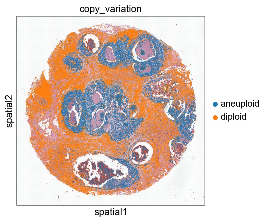
Copy number variation
This requires installation of CopyKAT and R environment in order to run the script. Here we simply show our result.
from thor.analy import prepare_and_run_copykat
prepare_and_run_copykat(adata,datadir, sam_name="BC")
[32]:
#sc.pl.spatial(ad, color='copy_variation', spot_size=50, ncols=1)

import seaborn as sns
import matplotlib.pyplot as plt
sc.set_figure_params(dpi=80, facecolor='white')

fig, ax = plt.subplots(figsize=(5,5))
sc.pl.spatial(ad, color='copy_variation', spot_size=50, vmax=4, cmap='viridis', img_key="hires", show=False, ax=ax)

ax.set_xticks([])
ax.set_yticks([])

plt.show()
Tertiary Lymphoid Structures(TLS) quantification
We use the list of 29 signature genes used by this study.
[33]:
# This is the gene list for the TLS score that we finally used, since it includes more related cell-type markers.
TLS_list_immunity = ['IGHA1',
                    'IGHG1',
                    'IGHG2',
                    'IGHG3',
                    'IGHG4',
                    'IGHGP',
                    'IGHM',
                    'IGKC',
                    'IGLC1',
                    'IGLC2',
                    'IGLC3',
                    'JCHAIN',
                    'CD79A',
                    'FCRL5',
                    'MZB1',
                    'SSR4',
                    'XBP1',
                    'TRBC2',
                    'IL7R',
                    'CXCL12',
                    'LUM',
                    'C1QA',
                    'C7',
                    'CD52',
                    'APOE',
                    'PLTP',
                    'PTGDS',
                    'PIM2',
                    'DERL3']

sc.tl.score_genes(ad, TLS_list_immunity, ctrl_size=len(TLS_list_immunity), gene_pool=None, n_bins=25, score_name='TLS_score_immunity', random_state=0, copy=False, use_raw=False)
[34]:
sc.set_figure_params(dpi=80, facecolor='white', frameon=False)


score = 'TLS_score_immunity'
ad1 = ad[ad.obs[score]>0.3]

scalefactor = ad.uns['spatial']['Visium_FFPE_Human_Breast_Cancer']['scalefactors']['tissue_hires_scalef']

fig, ax = plt.subplots(figsize=(6,6))

sc.pl.spatial(ad1, color=score, spot_size=50, cmap='viridis', ncols=1, ax=ax, show=False, title="", colorbar_loc=None)

tumor_borders = ad.uns['tumor_region_boundaries']
for name, border in tumor_borders.items():
    ax.plot(border[:,0]*scalefactor, border[:,1]*scalefactor, color='r', lw=0.5, zorder=3)


plt.show()
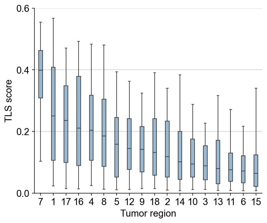
Rank the tumor regions according to the TLS score. We extended the tumor regions by 1 spot (55 um) outwards.
[35]:
region_col = 'tumor_region_ext'
import numpy as np
scores =  ['TLS_score_immunity']

for score in scores:
    ad1 = ad[ad.obs[score]>0.]
    TLS_clone_stats1 = ad1.obs.groupby(region_col)[[score]].aggregate('median')
    rank = list(np.array(TLS_clone_stats1.sort_values(by=score, ascending=False).index))
    rank.remove('0')

    print(rank)
['7', '1', '17', '16', '4', '8', '5', '12', '9', '18', '2', '14', '10', '3', '13', '11', '6', '15']
[36]:
import seaborn as sns
from matplotlib import pyplot as plt

sc.set_figure_params(dpi=80, facecolor='white')

tumor_col = 'tumor_region_ext'
score = 'TLS_score_immunity'

df = ad.obs[[region_col, score]]
df = df.loc[df[score]>0, :]
df = df.loc[df[region_col]!='0', :]

fig, ax = plt.subplots(figsize=(6, 5))

ax.spines.right.set_color('none')
ax.spines.top.set_color('none')
ax = sns.boxplot(df, y=score, x=region_col, whis=[5,95], dodge=False, width=0.3, fliersize=0., order=rank )
for patch in ax.patches:
    r, g, b, a = patch.get_facecolor()
    patch.set_facecolor((r, g, b, .5))
#sns.stripplot(df, y=score, x=region_col, ax=ax, size=0.8, jitter=0.05, dodge=True, legend="", alpha=1)
ax._remove_legend(ax.get_legend())
ax.set_ylim(0,0.6)
ax.set_yticks([0, 0.2, 0.4, 0.6])
ax.set_xlabel('Tumor region')
ax.set_ylabel('TLS score')
matplotlib.category - INFO - Using categorical units to plot a list of strings that are all parsable as floats or dates. If these strings should be plotted as numbers, cast to the appropriate data type before plotting.
matplotlib.category - INFO - Using categorical units to plot a list of strings that are all parsable as floats or dates. If these strings should be plotted as numbers, cast to the appropriate data type before plotting.
[36]:
Text(0, 0.5, 'TLS score')